3. Data Processing Basics¶

3.1. Calibrations¶

Master calibration reference (MasterCal) files are derived from calibration or science observations, and are used to remove the various components of the instrument signature from the data. Calibration exposures may combined or characterized to create a calibration, so that it may be applied when science data are processed. Some other instrument calibrations (e.g., slit mask definition files for MOS mode) have already been created for you by Gemini scientists, or are distributed with the gemini.f2 package.

3.1.1. Darks¶

Dark images are required for both imaging and spectroscopic observations, and show the spatially variable signal that accumulates during exposures in the absence of external illumination. This additive signal originates from multiple sources, including thermal radiation from both the shutter and the read-out electronics. The structure depends upon the exposure time and the read-out mode — i.e., the number of correlated double-sampled reads — for bright (1), medium (4), or faint (8).

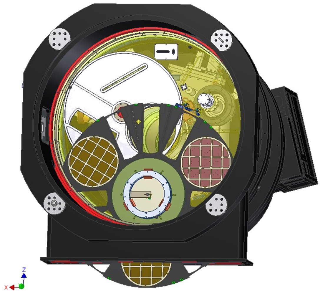
Dark MasterCal in false-color with log intensity stretch for exposures of 60s duration and READMODE = bright. Note the amplifier glow along the edges of the 32 sub-arrays of the detector. Click image to enlarge.

The dark correction is applied by simply subtracting the matching Dark MasterCal using either gemarith, or one of nireduce or nsreduce depending upon the observing configuration.

It is best to co-add several (10 or more) dark exposures, obtained on the same night, so that the noise in the Dark MasterCal does not dominate in science exposures with low background. The convention in the tutorials is to name the Dark MasterCal files MCdark_NNN where NNN is the exposure duration in seconds. The output Dark MasterCal file will have one FITS image extension, or 3 extensions if you elected to create the VAR and DQ arrays. Darks are the same for both imaging and spectroscopic observations.

3.1.2. Flat-Fields¶

Flatfields (required for both imaging and spectroscopy) are used to correct for differences in the sensitivities of pixels, to ensure that the same amount of illumination produces the same signal at all locations. Constructing a Flat-field MasterCal is largely a matter of combining dark-corrected flat-field exposures, with appropriate scaling, and outlier rejection. Flats for spectroscopy are obtained from observations of the GCAL continuum lamp, while imaging flats may be constructed from either lamp or night-sky observations. Separate flats must be created for each filter (imaging) or grism (spectroscopy); for MOS observations, separate flats are also required for each slit mask.

As with darks, it is best to combine a few to several well exposed flat-field exposures (if available) to keep noise in the flat-field from dominating the uncertainties in well exposed portions of the science data. The convention in the tutorials is to name the Flat MasterCal files MCflat_NNN where NNN is the name of the filter (imaging) or dispersing grism (spectroscopy).

3.1.2.1. Imaging Flats¶

GCAL imaging flats are usually created by subtracting exposures with the continuum lamp off from exposures with the lamp on. For K and Ks-band observations, however, the thermal emission is high and flats are made by subtracting dark exposures from exposures with the lamp off.

Flats can also be created from dark-subtracted sky exposures but, in these cases, it is necessary to mask objects before combining.

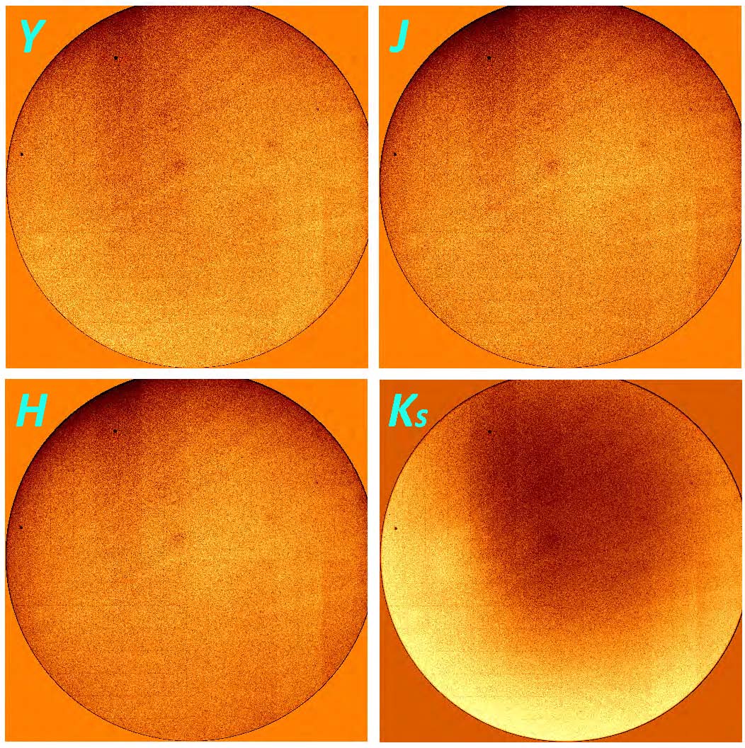
Imaging Flat-field MasterCals for the Y, J, H, Ks filters. This false-color rendering has a linear intensity stretch and a range of \(\pm30\) % (40% for Ks) about a mean of 1.0. Click image to enlarge.

3.1.2.2. Long-Slit Flats¶

Spectroscopic flatfields are created from dark-subtracted spectra of the GCAL continuum lamp. Rather than simply divide the science exposures by these flats, the variation in sensitivity with wavelength must first be removed. This is achieved by fitting a smooth function along the wavelength direction and dividing through by this function. See Flatfields for more details.

3.1.3. Wavelength Calibration¶

Spectroscopic observations only need to be wavelength calibrated. Exposures of an Argon arc lamp are used to determine the dispersion solution for spectroscopic modes. Arc lamp exposures should always be dark corrected and, while not essential, a flat-field correction typically improves the fit at the ends of the spectrum.

Individual arc lines are automatically identified based on their groupings and the estimated wavelength solution, and an analytic function (typically a 4th or 5th order polynomial) is fit for the wavelength as a function of pixel location. Once completed, the individual lines are then traced in the spatial direction to determine additional non-linearities. This information is attached to the science exposures with the gnirs.nsfitcoords task, and the transformations are performed by gnirs.nstransform.

3.1.4. Telluric Correction¶

Spectra of targets may need to be corrected for absorption by the Earth’s atmosphere (telluric absorption). This can be derived from telluric standards (stars that have few, relatively weak features in the IR), provided they are obtained at similar airmass close in time. In a similar matter to the spectroscopic flatfields, a smooth function is fit to the reduced, extracted spectrum of the standard (ignoring strongly absorbed regions) to produce the fractional absorption as a function of wavelength, and this is then applied to the science spectrum. This is performed by the task gnirs.nstelluric.

3.1.5. Night-sky frames¶

The night-sky background in the infrared is composed of emission lines and continuum, with the latter increasing strongly with wavelength. This background very often dominates the brightness of astrophysical targets, and it is variable on timescales of minutes. The thermal background from the telescope and instrument is also fairly strong in the K-band, but it is fairly stable.

The sky illumination in near-infrared images is determined by making sky frames. Multiple sky images at different locations are median-combined with objects masked out to produce an image devoid of astronomical sources. For crowded fields or very extended targets, these may require offset sky pointings; in sparse fields, a dither pattern is often used with small steps that move the target(s) around on the detector.

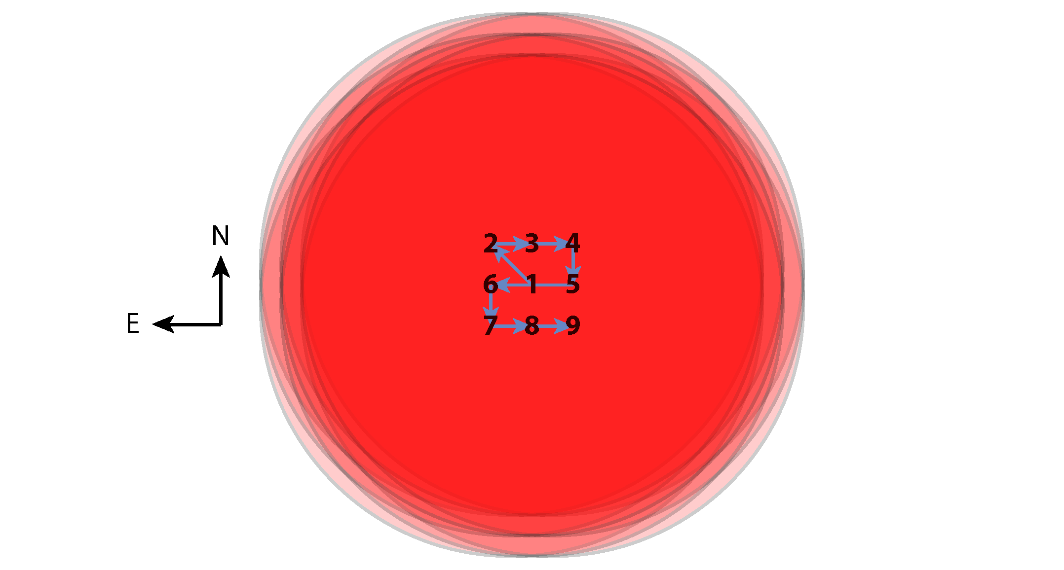
Nine-position dither pattern for IR imaging, for which offset exposures of equal duration are obtained sequentially in the serpentine order shown. Depth of combined exposure of the target field is represented by the intensity of the red colored area.

3.1.6. Flux Calibration¶

Flux calibration for imaging observations is performed using fully-reduced images of photometric standard stars, whose brightnesses have been accurately measured. Gemini keeps a List of Photometric Standards that are observed regularly to provide absolute photometric calibration of near-infrared images.

Spectrophotometric flux calibration is performed by dividing the fully-reduced spectrum of a star by a model representing its true spectrum in absolute flux density. This gives the factor for converting counts to flux density at each wavelength pixel, which can then be applied to the science spectrum.

At near-infrared wavelengths, there is little variation between the spectra of stars of a given spectral type, so almost any star can be used to perform this step. In practice, it is therefore possible to use the telluric standard as a spectrophotometric standard and combine the telluric correction and flux calibration into a single step.

3.2. Using the Python scripts¶

The python code on which the tutorials are based has dependencies on some common python packages, as listed in the table below:

**Python Package Dependencies**¶
File	Description
numpy	Numerical operations on arrays
astropy	General astronomical utilities including FITS I/O
yaml	Data serialization language for configuration files

These packages are included by default in the Anaconda distribution of python, which is highly recommended.

The reduction scripts are written as self-contained python programs, which can be executed in either of the following two ways:

python f2_reduce_images.py
./reduce_images.py

(the second will only work if the program has executable permission). A sensible way to run the reduction is one step at a time, commenting out the other steps, and examining the output before proceeding. For a more interactive session, you can choose to start up PyRAF (or python) and import the functions, which you will then be able to call directly:

% pyraf
--> from reduce_images import *

Each step of the data reduction is written as two python functions, typically appearing as

flat_dict = selectFlats(obslog)
reduceFlats(flat_dict)

The first of these queries the Observing Log to determine which unique flatfields can be made from the data, and which raw input frames and pre-existing calibrations (e.g., dark frames) are needed to make them. This is returned as a python dictionary in a format that can be passed to a function that performs the actual reduction by stringing together various IRAF tasks. This is somewhat inefficient from a coding perspective but it makes it much simpler to adapt the code by, for example, creating the dictionaries directly. Understanding python dictionaries will help you to get the most out of the scripts.

3.2.1. Python dictionaries¶

A python dictionary is an unordered list of pairs of keys and values. The reduction dictionary at each stage of processing contains entries where the key is the name of the output file, and the value is itself a dictionary describing the input files, with keys indicating the type of file and values giving the filenames. (For flatfield reduction, the bad pixel mask is included in the dictionary, even though it is an output file.)

If you are only reducing a small number of files, you may wish to make your dictionaries by hand to ensure maximum control over them. You initialize a dictionary as follows:

dict = {key1: value1, key2: value2, ...}

and add to or update it in either of the following ways:

dict[key3] = value3
dict.update({key3: value3, key4: value4, ...})

Let’s suppose you are reducing spectroscopic observations and you have the following data:

**Sample data**¶
Filenames	Type of data
S20180101S0001-S20180101S010	Darks
S20180101S0011-S20180101S020	GCAL flats
S20180101S0021	Arc

You can make the required python dictionaries as follows:

raw_darks = ['S20180101S{:04d}'.format(i) for i in range(1, 11)]
dark_dict = {'MCdark': {'input': raw_darks}}
raw_flats = ['S20180101S{:04d}'.format(i) for i in range(11, 21)]
flat_dict = {'MCflat': {'dark': 'MCdark',
                        'bpm': 'MCbpm',
                        'input': raw_flats}}
arc_dict = {'MCarc': {'dark': 'MCdark',
                      'bpm': 'MCbpm',
                      'flat': 'MCflat',
                      'input': ['S20180101S0021']}}

Note the input for the arc is a list, even though only a single file is being used. Also note how a list of consecutive filenames is constructed for the darks and flats, and how the second number is one more than the last frame to be included.

One final piece of good-to-know python information is that a statement is assumed to carry onto the next line of the file if any parentheses, brackets, or braces have not been closed.

Alternatively, you can write your reduction dictionaries in YAML and read them in using the syntax:

arc_dict = yaml.load(open('arc.yml', 'r'))

The YAML syntax for arc_dict in the above example should be written as shown below. Note that the input files must be presented as a list, one per line, preceded by a hyphen, even if there is only one input file, as in this example.

MCarc:
    dark:   MCdark
    flat:   MCflat
    bpm:    MCbpm
    input:
    - S20180101S0021

3.2.1.1. Task parameter files¶

PyRAF stores the parameters for the individual IRAF tasks as dictionaries. Each reduction step resets these parameters to their IRAF defaults with the unlearn() function and then reads in new values from a dictionary stored on disk as a yaml file. For example, the imgTaskPars.yml file starts like this:

f2prepare:
    rawpath: ./raw
    outprefix: p
    logfile: f2prepLog.txt

gemarith:
    fl_vardq: 'yes'
    logfile: gemarithLog.txt

The name of the task is given, followed by only the parameters that differ from the defaults (or whose values are most likely to have an effect on the final data products). Here, we are telling f2prepare that the raw files live in a subdirectory, and we wish to use the prefix p (rather than f) for prepared files, and log the task’s actions to a specific file.

The get_pars() function provided in the scripts performs several steps. First, it “unlearns” the specified tasks to set the parameter values back to their IRAF defaults. It then constructs dictionaries of overrides from the yaml file before returning them.

3.2.2. File naming conventions¶

The Gemini convention for naming output files is to prepend one or more characters to the input filename. This occurs for each intermediate stage of data reduction processing, and is summarized in the table below. Unfortunately the characters used are not entirely unique, so the meaning of a few of them must be derived from context.

**Processing Prefixes**¶
Prefix	Applies to:	Description
a	Spec	telluric correction applied
c	Spec	Flux calibrated
d	Img+Spec	Dark-subtracted
f	Img+Spec	Flatfielded
p	Img+Spec	Prepared
r	Img+Spec	Arbitrary reduction with nireduce/nsreduce
t	Spec	transformed (wavelength-calibrated rectilinear spectral image)
x	Spec	extracted 1-D spectra

During the processing, there will typically be a step where multiple input files are combined into a single output file. In such cases, the output file is normally given a completely new name. Where the output is a master calibration file, the style in the Tutorials is to use the format

MC <caltype> _ <config> .fits

where:

<caltype> is the type of calibration, e.g., dark or flat
<config> provides a unique configuration, the details of which will depend on the type of calibration. For a dark, this may simply be the exposure time, while for a flatfield it will be the filter. Additional information can be added, such as the date if separate calibrations are needed for each observing night.

For on-sky exposures of science targets or standard stars, a unique name should be given that will depend on the observing strategy.

3.3. Observing Log¶

How you organize your data is up to you and may depend on the number of files you have. The tutorials in this cookbook assume that you have created a working directory for the reduced files, with a single raw/ subdirectory into which all the raw files have been placed. In order to keep track of the files, it will be necessary to create an observing log that holds the important metadata for each file. The tutorials make use of this log to determine which files should be used at each stage of the reduction process in an automated manner.

3.3.1. Creating the Observing Log¶

A python script is provided that creates an observing log and writes it to disk as a FITS table. To use it:

Download obslog.py

Navigate to the raw/ subdirectory containing the raw files

Type python /path/to/obslog.py obslog.fits

The script opens the raw files in the directory in sequence and extracts relevant metadata from the primary header. The log can be viewed and edited with any software capable of handling FITS tables, such as TOPCAT. In addition to the columns containing the file metadata, there is a column titled use_me. This can be unchecked to remove files from consideration by the automated reduction steps in the tutorials.

3.3.2. Header Metadata¶

Values from the keywords listed below are harvested from the FITS headers. Some of the names are obscure, so they are re-mapped to somewhat more intuitive field names in the Observing Log. Fields may be added (or deleted: not recommended) by changing the KW_MAP definition at the top of the python script.

**Header Metadata**¶
Field name	Keyword	Description
use_me		Flag indicates file usage or exclusion (`True\|False`)
File		Filename (excluding `.fits`)
Object	`OBJECT`	Name of target
Filter	`FILTER`	Name of filter (imaging or blocking)
Disperser	`GRISM`	Name of dispersing element
ObsID	`OBSID`	Observation ID (e.g. GS-2018A-Q-1)
Texp	`EXPTIME`	Exposure time (in seconds)
Date		Date of observation start (YYYYMMDD)
Time	`TIME-OBS`	UT Time of observation start (HH:MM:SS.S)
RA	`RA`	Right Ascension of target (deg)
Dec	`DEC`	Declination of target (deg)
RA Offset	`RAOFFSET`	Offset in Right Ascension from target (arcsec)
Dec Offset	`DECOFFSE`	Offset in Declination from target (arcsec)
ObsType	`OBSTYPE`	Type of observation (e.g. `arc\|flat\|object`)
ObsClass	`OBSCLASS`	Class of observation: (e.g. `dayCal\|partnerCal\|science`)
Read Mode	`READMODE`	Detector readout Mode (`Bright\|Medium\|Dark`)
Reads	`LNRS`	Number of non-destructive reads
Coadds	`COADDS`	Number of array coadds
Mask	`MASKNAME`	Name for selected slit(mask)
MaskType	`MASKTYPE`	Type of mask (0=slit; 1=MOS; -1=pinholes)
Decker	`DECKER`	Decker position
GCAL Shutter	`GCALSHUT`	Position of GCAL shutter (`OPEN\|CLOSED`)
PA	`PA`	Position angle of instrument
Wavelength	`GRWLEN`	Grating approximate central wavelength (\(\mu\)m)
Airmass	`AIRMASS`	Airmass at time of observation

3.3.3. Using the Observing Log¶

The observing log can be queried in a simple manner by selecting observations whose metadata match supplied values. Specific examples are shown in the tutorials, but a brief reference is presented here. Some basic familiary with python is required.

The ObsLog class is defined at the start of each tutorial file, and is loaded with the syntax

obslog = ObsLog('path/to/obslog.fits')

To extract the metadata for a given file, use the syntax:

metadata = obslog['S20180101S0001']

Specific items of metadata can be extracted with:

t = obslog['S20180101S0001']['Texp']
t, obstype = obslog['S20180101S0001']['Texp', 'ObsType']

To find observations that match a specific set of metadata, construct a python dictionary indicating the required matches, e.g.,

qd = {'ObsType': 'DARK', 'Texp': 5}
matching = obslog.query(qd)

will return all rows containing 5-second dark exposures. To return only the filenames of these exposures, use:

darkfiles = obslog.file_query(qd)

To select observations from a particular UT date, or between two (inclusive) dates, use:

matching = obslog.query({'Date': '20180101'})
matching = obslog.query({'Date': '20180101:20180103'})

Finally, the first and last keywords can be used to select the first and last filenames, e.g.,

qd = {'ObsType': 'FLAT', 'Texp': 10, 'first': 'S20180101S0020',
      'last': 'S201801020355'}
files = obslog.file_query(qd)

will return the filenames of all 10-second flatfield exposures in the range specified.

An additional python function, merge_dicts(), is provided to assist with the construction of queries. It takes two dictionaries as arguments and returns a single dictionary by using the second dictionary to add new entries (only if allow_new=True) or update existing entries in the first dictionary.

3.3.3.1. Advanced Usage¶

The ObsLog class simply allows a very limited number of simple methods on a data table. Queries return another table, which can be used to instantiate a new observation log, e.g.,

obslog_night1 = ObsLog(obslog.query({'Date': '20180101'}))

For queries that are more complicated than simple matching, the table itself is accessible as the table attribute of the log. For example, suppose you want to select all science exposures with offset distances greater than 60 arcseconds:

# Extract offset information
raoff, decoff = obslog.table['RA Offset'], obslog.table['Dec Offset']
distance_squared = raoff*raoff + decoff*decoff
# Make a new log of objects more than 60 arcseconds away
newlog = ObsLog(obslog.table[distance_squared > 3600])
# Now query this log
distant_files = newlog.file_query({'ObsClass': 'science'}))