4. F2 Imaging Tutorial

Note

We strongly recommend that you reduce your F2 imaging data with DRAGONS (Data Reduction for Astronomy from Gemini Observatory North and South) rather than PyRAF. DRAGONS is simpler to use and provides genuine pipeline capabilities. A tutorial is available at https://dragons.readthedocs.io/projects/f2img-drtutorial/en/stable/

The recipe described here provides a recommended, but not unique path for processing your FLAMINGOS-2 science data.

This tutorial will use observations from program GS-2013B-Q-15 (PI:Leggett), NIR photometry of the faint T-dwarf star WISE J041358.14-475039.3, obtained on 2013-Nov-21. Images of this sparse field were obtained in the Y,J,H,Ks bands using a dither sequence; dayCal darks and GCAL flats were obtained as well. Leggett, et al. (2015; [L15]) briefly describe the data reduction procedures they followed, which are similar to those described below.

4.1. Retrieving the Data

The first step is to retrieve the data from the Gemini Observatory Archive (see Archive Searches). The observations of this target were taken with a single Observation ID, so it is possible to obtain all the science exposures with a single query:

https://archive.gemini.edu/searchform/GS-2013B-Q-15-39

After retrieving the science data, click the Load Associated Calibrations tab on the search results page and download the associated dark and flat-field exposures.

If you look carefully, you will note that each set of flatfields comprises 6 frames from 2013-Nov-26 and 4 from 2013-Nov-29. F2 flats are typically done in sets of 12 (6 each of lamp-on and lamp-off, except for the K band), so the fact that the archive search has had to use observations from two different nights indicates a problem. Better is to use the flatfields from the later night, and these can be retrieved with the following URL:

https://archive.gemini.edu/searchform/F2/imaging/20131129/FLAT

The flats from 2013-Nov-26 (the only files from this date) can be deleted from disk in the normal way:

rm S20131126*

You will also note that there some pre-reduced calibrations exist in the archive. These are identified with the original name of the first file and a suffix indicating the type of calibration, e.g., S20140124S0093_dark.fits. These can be left as the observing log will only include raw files.

4.1.1. Exposure Summary

The data contain exposures of a specific science target and dayCal calibrations; see the table below for a summary. The science exposures were obtained in a \(3\times3\) spatial dither pattern, with a spacing of about 15 arcsec in each direction from the initial alignment (see Night-sky frames).

Exposure Summmary

Target	Filter	T_exp	N_exp
WISE 0413-4750	Y	120	9
	J	60	9
	H	15	72
	Ks	15	72
Dark		120	10
		60	21
		20	20
		15	10
		8	24
		3	13
GCAL Flat	Y	20	12 (6 on + 6 off)
	J	60	12 (6 on + 6 off)
	H	3	12 (6 on + 6 off)
	Ks	8	6 (off)

Note that dark exposures have been taken with exposure times that match not just the science exposures, but also the flatfields. Darks for F2 are usually taken in groups of 10, and you may choose to use only the 10 darks taken closest in time to the relevant exposure; if so, you can either delete the additional exposures now or uncheck the use_me flag after creating the observing log.

4.2. Preparation

First download obslog.py to the raw subdirectory and create an observing log, as described in Observing Log.

python obslog.py obslog.fits

The other files needed for this tutorial are a python script and two configuration files.

• Download: reduce_images.py

This python script will perform an automated reduction of the WISE 0413-4750 data; see the section Using the Python scripts to understand how to use it. This tutorial will take you through it, step by step, so you can understand the procedure and how to edit it for your own F2 imaging data, should you choose to do so.

Configuration files are required for the IRAF task parameters that differ from the defaults, and to provide the script with information about the targets.

• Download IRAF task parameters: imgTaskPars.yml
• Download target information: imgTargets.yml

4.2.1. Target configuration file

Each entry in this file gives the name (or root name) of the output file, and is followed by a list of parameters that will query the observation log to produce the list of science input frames. In addition, a parameter groupsize can be added, which will break the list of science frames into groups of this size, each of which is reduced independently (see Science targets for more details). Note that, because only one object has been observed in this program, only the filter needs to be specified in the configuration file. Since all exposures were taken on the same night, we use the default global darks, flats, and BPMs, and do not need to specify them in the file.

Y0413:
    Filter: Y

J0413:
    Filter: J

H0413:
    Filter: H
    groupsize: 9

K0413:
    Filter: Ks
    groupsize: 9

4.2.2. Configuration of nireduce

The nireduce task has several parameters; the table below lists the defaults for the processing flags — i.e., the parameters with logical values to indicate whether to perform an operation.

nireduce Processing Flag Defaults

Flag	Default	Description
fl_autosky	No	Determine constant sky level to restore?
fl_dark	Yes	Subtract dark image?
fl_flat	No	Apply flat-field correction?
fl_scalesky	Yes	Scale the sky image to input image?
fl_sky	No	Perform sky subtraction using skyimage?
fl_vardq	Yes	Propagate VAR and DQ extensions?

The parameter values need to be chosen carefully, as the order of operations performed by the task is not consistent with the order adopted in this tutorial. For example, nireduce performs sky subtraction before flatfielding when both are selected, requiring the sky frame to not have been flatfielded, but this is not ideal for two reasons: it is difficult to determine how well objects have been removed from the sky frame without it having been flatfielded, and scaling is less reliable when the background counts are not uniform across the image. Therefore nireduce will be invoked multiple times, with different processing flag settings, to accomplish the processing steps in the needed order. Also, the simple process of subtracting a dark frame will be performed with the gemarith task, rather than nireduce.

4.3. Darks

Dark MasterCals are produced by combining individual dark frames. The function selectDarks() automatically produces lists of all dark frames of the same exposure time by querying the observing log.

def selectDarks(obslog):
    dark_dict = {}
    qd = {'ObsType': 'DARK'}
    exptimes = set(obslog.query(qd)['Texp'])
    for t in exptimes:
        darkFiles = obslog.file_query(merge_dicts(qd, {'Texp': t}))
        outfile = 'MCdark_'+str(int(t))
        dark_dict[outfile] = {'input': darkFiles}
    return dark_dict

This works by first querying the observing log for all dark frames. With the query dictionary qd = {'ObsType': 'DARK'}, obslog.query(qd) returns all rows in the observing log corresponding to dark frames. obslog.query(qd)['Texp'] returns the exposure times of these frames, and the set() function collapses this down to a list of unique values.

Then there is a loop over each unique exposure time, with the observing log being queried for the names of files that are darks and have the correct exposure time. An entry is placed in dark_dict with an appropriately-named output file and the list of all raw dark frames. The exposure time is coerced to an integer because PyRAF has issues if there is a . in the name of a file.

There is also a function, nightlyDarks(), that will separate the darks by observation date (actually, the first 8 digits from the original filename) as well as exposure time, which you might wish to do for your data (e.g., if you have observations, and darks, widely separated in time). This produces filenames like MCdark_20180101_5.fits, and you will have to adapt the subsequent code to select the correct one.

def reduceDarks(dark_dict):
    prepPars, combPars = get_pars('f2prepare', 'gemcombine')
    for outfile, file_dict in dark_dict.items():
        darkFiles = file_dict['input']
        for f in darkFiles:
            f2.f2prepare(f, **prepPars)
        if len(darkFiles) > 1:
            gemtools.gemcombine(filelist('p', darkFiles), outfile,
                                **darkCombPars)
        else:
            iraf.imrename('p'+darkFiles[0], outfile)
    iraf.imdelete('pS*.fits')

Reduction of the dark frames is straightforward: they are prepared and then combined. If only one dark frame is sent, then it is simply renamed after being prepared.

4.4. Flatfields

Flatfield frames can be constructed either from observations of the calibration (GCAL) lamp, or from images of the sky (with the removal of astronomical objects).

4.4.1. GCAL Flats

As discussed in Flat-Fields, GCAL flats normally consist of observations of equal time taken with the shutter open (“lamp-on”), and with the shutter closed (“lamp-off”). For the K and Ks filters, only closed-shutter flats are taken and dark frames are subtracted from these.

def selectGcalFlats(obslog):
    qd = {'ObsType': 'DARK'}
    tshort = min(obslog.query(qd)['Texp'])
    shortDarks = obslog.file_query(merge_dicts(qd, {'Texp': tshort}))

    flat_dict = {}
    qd = {'ObsType': 'FLAT'}
    params = ('Filter', 'Texp')  # Can add 'Date'
    flatConfigs = unique(obslog.query(qd)[params])
    for config in flatConfigs:
        filt, t = config
        config_dict = dict(zip(params, config))
        if filt.startswith('K'):
            lampsOn = obslog.file_query(merge_dicts(qd, config_dict))
            lampsOff = obslog.file_query({'ObsType': 'DARK', 'Texp': t})
        else:
            config_dict['GCAL Shutter'] = 'OPEN'
            lampsOn = obslog.file_query(merge_dicts(qd, config_dict))
            config_dict['GCAL Shutter'] = 'CLOSED'
            lampsOff = obslog.file_query(merge_dicts(qd, config_dict))
        bpmFile = 'MCbpm_'+filt+'.pl'
        outfile = 'MCflat_'+filt
        flat_dict[outfile] = {'bpm': 'MCbpm_'+filt+'.pl',
                              'lampsOn': lampsOn, 'lampsOff': lampsOff,
                              'shortDarks': shortDarks}
    return flat_dict

The niflat task produces a bad pixel mask as well as the flatfield. In order to do this, it needs short-exposure darks, so the observation log is first queried for all the exposure times of all the dark frames; the lowest of these is determined and a second query made to find the list of dark files matching this exposure time.

The observation log is queried for flatfield images and the configurations of these (here the combination of filter and exposure time) are whittled down to a list of unique pairs – note that the unique() function must be used instead of set() when more than one field is being extracted from the log. For each configuation, the observation log is then queried two more times, to separate the lamp-on and lamp-off flats. For most filters, this is done by searching for flats with the appropriate combination of filter and exposure time, and the GCAL shutter either open or closed; for K and Ks, any flats are selected as lamp-on, while dark exposures of the same exposure time are used for the lamp-off exposures.

An entry in the reduction dictionary is then created, keyed by the name of the output file. Its value is a dictionary with the name of the output BPM file, and lists of the lamp-on and lamp-off files, and a list of the short-exposure darks.

4.4.2. Sky flats

Flatfields can also be made from the twilight sky. The same reduction dictionary format is used, but the sky images take the place of the lamp-on frames, and darks of the same exposure time are used in place of the lamp-off frames. The short darks are identified and used in exactly the same way as above.

def selectSkyFlats(obslog):
    qd = {'ObsType': 'DARK'}
    tshort = min(obslog.query(qd)['Texp'])
    shortDarks = obslog.file_query(merge_dicts(qd, {'Texp': tshort}))

    flat_dict = {}
    qd = {'Object': 'Twilight'}
    params = ('Filter', 'Texp')
    flatConfigs = unique(obslog.query(qd)[params])
    for config in flatConfigs:
        filt, t = config
        config_dict = dict(zip(params, config))
        lampsOn = obslog.file_query(merge_dicts(qd, config_dict))
        lampsOff = obslog.file_query({'ObsType': 'DARK', 'Texp': t})
        bpmFile = 'MCbpm_'+filt+'.pl'
        outfile = 'MCflat_'+filt
        flat_dict[outfile] = {'bpm': 'MCbpm_'+filt+'.pl',
                              'lampsOn': lampsOn, 'lampsOff': lampsOff,
                              'shortDarks': shortDarks}
     return flat_dict

4.4.3. Creating the flatfields

The same function is used to create the flatfields, irrespective of whether they are GCAL flats or sky flats, with the value of the boolean gcal parameter indicating the type of flats, since this affects the parameters for the niflat task.

def reduceFlats(flat_dict, gcal=True):
    prepPars, flatPars = get_pars('f2prepare', 'niflat')
    prepPars['fl_nonlinear'] = 'no'        # Fudge to fix (slightly)
    flatPars['key_nonlinear'] = 'SATURATI' # over-exposed flats
    if not gcal:
        flatPars.update({'fl_rmstars': 'yes', 'scale': 'median'})
    for (outfile, bpmFile), (lampsOn, lampsOff,
                             shortDarks) in flat_dict.items():
        for f in shortDarks+lampsOn+lampsOff:
            if not os.path.exists('p'+f+'.fits'):
                f2.f2prepare(f, **prepPars)
        flatPars.update({'darks': filelist('p', shortDarks),
                           'lampsoff': filelist('p', lampsOff),
                           'flatfile': outfile, 'bpmfile': bpmFile})
        niri.niflat(filelist('p', lampsOn), **flatPars)
    iraf.imdelete('pS*.fits')

The default gcal=True assumes that the flatfields are GCAL flats, so should be combined directly without scaling; if gcal=False, then the images are scaled to the same median and stars are identified and removed.

The 8-second exposure time chosen for the Ks flats causes pixels in the bottom-left quadrant of the detector to creep into the non-linear regime, and they will therefore be flagged during preparation and flatfield creation. In practice, we do not want this to happen, so we choose not to flag non-linear pixels in f2prepare, and ignore them when making the flatfield by telling niflat that the non-linearity threshold is actually the saturation level. Once the detector properties of F2 were better determined, shorter flatfield exposures were taken and this fudge should not be needed for more recent data. Those two lines should be removed if the illumination level of your flats is within acceptable limits.

Since the short darks will be the same for all images, we check whether the prepared files are already on disk before calling f2prepare. The parameters for niflat are then updated with the lists of prepared input files and the task is executed.

4.5. Science targets

Depending on your scientific aims and observing strategy, there are many ways that the science frames could be combined; for example, you may wish to combine all the images in a given filter together into a single output image, or you may be looking for variability and so want to produce multiple output images. In addition, you may be observing a sparse field where a sky frame can be created from the observations of the target, or you may need to take sky frames at offset positions. For this reason, and to provide flexibility, the dictionary detailing how to produce the science images is constructed with the help of a Target configuration file.

There is a single function that constructs dictionaries for both the science output images and the sky frames.

def selectTargets(obslog):
    with open('imgTargets.yml', 'r') as yf:
        targets = yaml.load(yf)
    sci_dict = {}
    qd = {'ObsClass': 'science'}
    for outfile, pars in targets.items():
        sciFiles = obslog.file_query(merge_dicts(qd, pars))
        t, filt = obslog[sciFiles[0]]['Texp', 'Filter']
        file_dict = {'dark': pars.get('dark', 'MCdark_'+str(int(t))),
                     'bpm': pars.get('bpm', 'MCbpm_'+filt),
                     'flat': pars.get('flat', 'MCflat_'+filt),
                     'sky': pars.get('sky', 'self')}
        try:
            groupsize = pars['groupsize']
        except:
            sci_dict[outfile] = merge_dicts(file_dict, {'input': sciFiles})
        else:
            index = 1
            while len(sciFiles) > 0:
                sci_dict['{}_{:03d}'.format(outfile, index)] = merge_dicts(
                    file_dict, {'input': sciFiles[:groupsize]})
                del sciFiles[:groupsize]
                index += 1
    # Create list of sky frames used in reduction
    sky_list = [v['sky'] for v in sci_dict.values()]
    # Make a reduction dict of bespoke skies
    sky_dict = {k: v for k, v in sci_dict.items() if k in sky_list}
    # And then remove these from the science reduction dict
    sci_dict = {k: v for k, v in sci_dict.items() if k not in sky_list}
    return sky_dict, sci_dict

The configuration file is opened and each entry processed by first constructing a list of input science frames using the query parameters provided in this file. It is assumed that these frames all have the same exposure time and filter, so these properties are determined from the first frame in the list. The exposure time is used to determine the name of the MasterCal Dark, and the filter is used to determine the names of the MasterCal Flat and MasterCal BPM, if these are not explicitly provided in the file.

Each entry can have an optional sky parameter. This can have the value none (indicating no sky-subtraction is required, e.g., for short-exposure standard stars) or the name of a specific file. It can be absent for two reasons: either this output image is a sky frame to be subtracted from another science frame, or a sky frame should be constructed from the same science frames. If absent, the word self is used as a placeholder.

In principle, we’re now good to go, but it may be desirable to group the input files up into more manageable chunks. This is indicated in the Target configuration file by the use of a groupsize entry. If absent, a single entry is created in the science reduction dictionary, containing all the science input files. If this key does exist, however, then the input file list is broken up, groupsize files at a time, to produce separate entries in the reduction dictionary (all using the same MasterCals), until there are no files left. The output filenames are given suffixes _001, _002, etc. Grouping the images in this way copes with variations in the sky better, and also means a problem during the coaddition of the frames won’t affect the entire output.

At this stage, the reduction dictionary may include bespoke sky frames, which need to be separated since they will be reduced differently (and also need to be reduced before the science frames for which they are used). A list the sky frames is extracted from the reduction dictionary, and any entries with output files matching an entry in this list are placed in their own dictionary and removed from the science dictionary. The function returns both dictionaries for processing.

4.5.1. Bespoke sky images

The construction of sky images is straightforward with the task nisky, which performs a two-pass procedure to mask objects from the images before combining them.

def reduceSkies(sky_dict):
    prepPars, redPars, skyPars = get_pars('f2prepare', 'nireduce', 'nisky')
    for outfile, file_dict in sky_dict.items():
        darkFile = file_dict['dark']
        prepPars['bpm'] = file_dict['bpm']
        flatFile = file_dict['flat']
        skyFiles = file_dict['input']
        for f in skyFiles:
            f2.f2prepare(f, **prepPars)
            gemtools.gemarith('p'+f, '-', darkFile, 'dp'+f, **arithPars)
        skyPars['outimage'] = 'nf_'+outfile
        niri.nisky(filelist('dp', skyFiles), **skyPars)
        redPars.update({'fl_dark': 'no', 'fl_flat': 'yes',
                        'flatimage': flatFile, 'outimage': outfile})
        niri.nireduce('nf_'+outfile, **redPars)
        iraf.imdelete('nf_'+outfile)
    iraf.imdelete('pS*.fits')

The input images have to be prepared and dark-subtracted before being sent to nisky. Note that the output sky frame is not flatfielded, so we have to flatfield it in order to ascertain how well the object masking has worked. The dark-subtracted files are deliberately not removed from disk by this function; if the sky is being constructed from dithered images of a science target, they will be used for the reduction of the science image.

4.5.2. Science images

The final science data products are constructed from the science reduction dictionary. The precise series of reduction steps depends on the manner in which sky-subtraction is to be performed (if at all) and so there are logic-dependent blocks in the tutorial code that may be irrelevant for your own dataset.

def reduceScience(sci_dict):
    prepPars, arithPars, redPars, coaddPars = get_pars('f2prepare', 'gemarith',
                                                       'nireduce', 'imcoadd')
    for outfile, file_dict in sci_dict.items():
        darkFile = file_dict['dark']
        prepPars['bpm'] = file_dict['bpm']
        flatFile = file_dict['flat']
        skyFile = file_dict['sky']
        sciFiles = file_dict['input']
        if skyFile == 'self':
            # Make the sky (also leaves dark-subtracted files on disk)
            skyFile = outfile+'_sky'
            reduceSkies({skyFile: file_dict})
        else:
            for f in skyFiles:
                f2.f2prepare(f, **prepPars)
                gemtools.gemarith('p'+f, '-', darkFile, 'dp'+f, **arithPars)
        redPars.update({'outprefix': 'f', 'fl_sky': 'no',
                        'flatimage': flatFile})
        niri.nireduce(filelist('dp', sciFiles), **redPars)
        imcoadd_infiles = filelist('fdp', sciFiles)
        if skyFile != 'none':
            redPars.update({'outprefix': 'r', 'fl_flat': 'no',
                            'fl_sky': 'yes', 'skyimage': skyFile})
            niri.nireduce(filelist('fdp', sciFiles), **redPars)
            imcoadd_infiles = filelist('rfdp', sciFiles)
        coaddPars.update({'badpixfile': bpmFile, 'outimage': outfile})
        gemtools.imcoadd(imcoadd_infiles, **coaddPars)
    iraf.imdelete('pS*.fits,dpS*.fits,rdpS*.fits,rfdpS*.fits')

Each entry in the science reduction dictionary is reduced in turn. If the sky frame is to be constructed from the science frames themselves (i.e., the entry has self instead of a filename), then reduceSkies() is called to produce that frame, which is named after the science output file but given the suffix _sky. This will leave the individual dark-subtracted files on disk which can be used for the next steps; otherwise, the files must be prepared and dark-subtracted.

The individual science frames are then flatfielded, and sky-subtraction takes place if requested. Note that, if no sky-subtraction is to take place (e.g., for short exposures of photometric standards) the fl_sky parameter for nireduce has to be explicitly set to no (even though that is the default) in case a previous iteration of the loop had changed its value. Finally, the reduced files are sent to imcoadd to be aligned and stacked.

Caution

imcoadd can be quite fickle, especially when there are artifacts in the data such as caused by the peripheral wavefront sensor guide probe. It is recommended that you run the task interactively and check each coordinate fit (by pressing x and y once the interactive fitting window appears) to confirm that the points scatter around zero and have an rms of a few tenths of a pixel.

An additional function, coaddScience() is provided in the tutorial script. If you find you are having problems with imcoadd, it can be frustrating and time-consuming to have to go back to the raw data and perform the standard reduction steps again, and you may wish to fully reduce the individual files but not combine them at this stage. Simply comment out the call to imcoadd and remove the appropriate files from the deletion list in the next line to ensure they remain on disk. Then call coaddScience() with the appropriate science reduction dictionary to complete the reduction.

If you have broken your list of science files into groups then neither reduceScience() nor coaddScience() will combine these groups. You will need to make a final call to imcoadd with the separate stacks if you wish to have a single stacked output image.

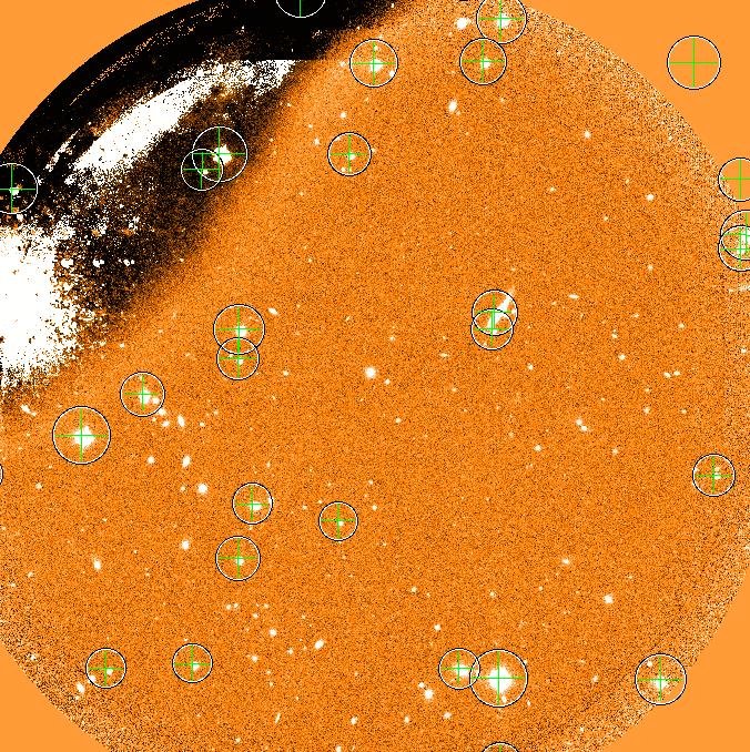
Y-band image produced by this tutorial, with locations of stars from the 2MASS catalog indicated. Note the slight astrometric offset and the effect of the peripheral wavefront sensor in the top left of the image.

4.6. Astrometric calibration

The astrometry given in the image headers should be accurate enough to allow you to identify your target(s) in the image, but there may be an offset of a few arcseconds. The simplest way to correct for this offset is by using an image display tool to measure the pixel coordinates of an objects whose celestial coordinates you know (e.g., from a catalog). You can then update the world coordinate system with the following four IRAF/PyRAF commands:

hedit image[SCI] CRPIX1 x
hedit image[SCI] CRPIX2 y
hedit image[SCI] CRVAL1 ra
hedit image[SCI] CRVAL2 dec

where x and y are the pixel coordinates, and ra and dec the celestial coordinates (in degrees) of the object.

Alternatively, or if you require a more accurate WCS, you can try one of the following options:

• the IRAF MSCRED package
• the astrometric calibration tools in Gaia (part of the Starlink Software)
• astrometry.net

4.7. Flux calibration

The reduced images of your science target(s) and standard star(s) are in ADUs per exposure. After measuring the brightness of both objects in these units, the magnitude of your science target is simply given by:

\[m_{sci} = m_{std} - 2.5 \log_{10} \frac{c_{sci} / t_{sci}}{c_{std} / t_{std}}\]

where \(m_{std}\) is the magnitude of the standard star in the filter used; \(c_{sci}\) and \(c_{std}\) are the summed counts for the science target and standard, respectively; and \(t_{sci}\) and \(t_{std}\) are the exposure times of each individual frame used when observing the science target and standard.

This calculation will only be accurate if both objects were observed in clear skies (CC50) and at similar airmasses. The atmospheric extinction in the near-infrared is small at Cerro Pachon so a modest difference in airmasses is unlikely to affect the accuracy of the final result. If you require photometric accuracy greater than a few per cent, it is necessary to either calibrate the photometry directly from sources in the image or observe bespoke photometric standards.