5. F2 Longslit Tutorial

The recipe described here provides a recommended, but not unique path for processing your FLAMINGOS-2 science data.

This tutorial will use observations from program GS-2014B-Q-17 (PI:Leggett), longslit spectra of the faint Y1 star WISE J035000.32-565830.2, obtained between 20 14-Nov-07 and 2014-Dec-04. The spectra were obtained with the 4-pixel wide (0.72 arcsec) slit and the JH grism at \(1.4\mu m\). Telluric standards were included in the observing plan, as were Ar comparison arcs. Leggett et al. (2016; [L16]) describe the data reduction procedures they followed, which are very similar to those described below.

5.1. Retrieving the Data

The first step is to retrieve the data from the Gemini Observatory Archive (see Archive Searches). The observations we are interested in are part of a larger program with multiple targets, so we only wish to obtain the observations in a particular date range.

https://archive.gemini.edu/searchform/GS-2014B-Q-17/spectroscopy/20141107-20141231/

After retrieving the science data, click the Load Associated Calibrations tab on the search results page and download the associated dark and flat-field exposures. Calibrations are found many days either side of the actual science exposures and so it is worthwhile looking at the dates of the calibrations and removing some of the more distant ones (e.g., there are 6 flats from early October 2014, one from 29 Dec, and two from January 2015).

5.1.1. Exposure Summary

The data contain exposures of a specific science target, telluric standards, and dayCal calibrations that are summarized in the table below. It is important to review the observing log database to understand how to approach the data processing. All exposures were obtained with ReadMode = Bright.

Exposure Summmary

Target	T_exp	N_exp	Date
WISE 0350-56	300	52	2014-Nov-07
	300	6	2014-Nov-13 (not used)
	300	16	2014-Dec-04
HD 13517 (F3V)	5	8	2014-Nov-07
HD 17813 (F2V)	5	8	2014-Nov-13 (not used)
HD 30526 (F7V)	5	4	2014-Nov-07
HD 36636 (F3V)	5	4	2014-Dec-04
Dark	300	24	2014-Nov-08 — 2014-Dec-13
	15	27	2014-Nov-08 — 2014-Dec-13
	5	27	2014-Nov-08 — 2014-Dec-13
	4	21	2014-Nov-08 — 2014-Dec-13
GCAL Flat	4	10	2014-Nov-05 — 2014-Dec-15
GCAL Ar Arc	15	3	2014-Nov-07 — 2014-Dec-04

5.2. Preparation

First download obslog.py to the raw subdirectory and create an observing log, as described in Observing Log.

python obslog.py obslog.fits

The other files needed for this tutorial are a python script and two configuration files.

• Download: reduce_ls.py

This python script will perform an automated reduction of the spectroscopy of WISE J0350; see the section Using the Python scripts to understand how to use it. This tutorial will take you through it, step by step, so you can see understand the procedure and how to edit it for your own F2 longslit data, should you choose to do so.

Configuration files are required for the IRAF task parameters that differ from the defaults, and to provide the script with information about the targets.

• Download IRAF task parameters: lsTaskPars.yml
• Download target information: lsTargets.yml

5.2.1. Target configuration file

In order to process the observations of celestial targets (both telluric and/or spectrophotometric standards and science targets), it is necessary to prepare a file describing the ways in which the files should be combined. For the tutorial, you should download lsTargets.yml

The contents of this file are as follows:

HD13517:
    Object:    HD 13517
    Date:      '2014-11-07'
    arc:       arc_S20141107S0235

HD30526:
    Object:    HD 30526
    Date:      '2014-11-07'
    arc:       arc_S20141107S0263

HD36636:
    Object:    HD 36636
    Date:      '2014-12-04'
    arc:       arc_S20141204S0075
    nsreduce:
        skyrange:  90

epoch1:
    first:     S20141107S0207
    last:      S20141107S0234
    arc:       arc_S20141107S0235
    telluric:  HD13517

epoch2:
    ObsID:     GS-2014B-Q-17-62
    first:     S20141107S0239
    arc:       arc_S20141107S0263
    telluric:  HD30526

epoch3:
    Date:      '2014-12-04'
    arc:       arc_S20141204S0075
    telluric:  HD36636

The order of entries is irrelevant, but each entry is labeled with an output filename, and information that will allow the construction of a dictionary with which to query the observation log to produce a list of input files. There are several ways to do this, including specifying the first and last filenames, or the date, or the Observation ID.

Note

If you are selecting by a single date, the date string must be enclosed in quoted to prevent it being parsed into a python date object.

In addition, the name of a wavelength calibration (the output file from nswavelength) must be provided, and a telluric absorption standard if one is to be used. The keywords dark, flat, and bpm can also be used to specify additional calibration files, if the default choices are inappropriate. Finally, additional parameters for nsreduce and/or nsextract can also be given as indicated.

More details about this file are given in the sections on Telluric standards and Science targets, where it is used.

5.2.2. Configuration of nsreduce

The nsreduce task has several parameters; the table below lists the defaults for the processing flags — i.e., the parameters with logical values to indicate whether to perform an operation.

nsreduce Processing Flag Defaults

Flag	Default	Description
fl_cut	Yes	Cut images using F2CUT?
fl_process_cut	Yes	Cut the data before processing?
fl_nsappwave	Yes	Insert approximate wavelength WCS keywords into header?
fl_dark	No	Subtract dark image?
fl_save_dark	No	Save processed dark files?
fl_sky	No	Perform sky subtraction using skyimages?
fl_flat	Yes	Apply flat-field correction?
fl_vardq	Yes	Propagate VAR and DQ?

The parameter values need to be chosen carefully, as the order of operations performed by the task is not consistent with the order adopted in this tutorial. This means nsreduce will be invoked multiple times, with different flag settings, to accomplish the processing steps in the needed order.

5.3. Darks

Since dark frames are the same irrespective of whether they are used for imaging or spectroscopic observations, the procedure for reducing them is identical to that described in the Imaging Tutorials’ section on Darks.

5.4. Flatfields

Construction of the MasterCal Flats follows the same pattern as the darks, first constructing a dictionary with one entry for each output image, and then processing the entries in this dictionary.

def selectFlats(obslog):
    flat_dict = {}
    qd = {'ObsType': 'FLAT'}
    params = ('Texp', 'Disperser')
    flatConfigs = unique(obslog.query(qd)[params])
    for config in flatConfigs:
        t, grism = config
        config_dict = dict(zip(params, config))
        flatFiles = obslog.file_query(merge_dicts(qd, config_dict))
        outfile = 'MCflat_'+grism
        flat_dict[outfile] = {'dark': 'MCdark_'+str(int(t)),
                              'bpm': 'MCbpm_'+grism+'.pl',
                              'input': flatFiles}
    return flat_dict

While the only thing that matters for dark frames is the exposure time, for flatfields it is the combination of disperser (grism) and filter (the central wavelength of the F2 grisms is not configurable). However, in practice there is a natural choice of filter for each of the grisms so only this is used to identify and name the flatfields. In addition, the exposure time must be determined so the appropriate dark exposure can be subtracted (while flats do not need to have the same exposure time to be combined, the illumination is constant so in practice this is always the case).

A list of unique combinations of exposure time and grism are extracted from the observing log (the function unique() is used rather than set() when more than one column is used) and then these are cycled through to build a dictionary. For each output flatfield (named according to the grism used), the dictionary entry has the MasterCal dark, the output bad pixel mask, and the list of raw input frames.

Note

The output flatfields and BPMs are only distinguished by the name of the grism. If you were to take flats with the same grism but different filters, the software would crash as it attempts to create the same files the second time around. It is up to you to ensure that the output filenames for each set of MasterCal files are unique.

def reduceFlats(flat_dict, pars):
    prepPars, arithPars, cutPars, flatPars = get_pars('f2prepare', 'gemarith',
                                                      'f2cut', 'nsflat')
    for outfile, file_dict in flat_dict.items():
        darkFile = file_dict['dark']
        bpmFile = file_dict['bpm']
        flatFiles = file_dict['input']
        for f in flatFiles:
            f2.f2prepare(f, **prepPars)
            gemtools.gemarith('p'+f, '-', darkFile, 'dp'+f, **arithPars)
            f2.f2cut('dp'+f, **cutPars)
        flatPars.update({'flatfile': outfile, 'bpmfile': bpmFile})
        gnirs.nsflat(filelist('cdp', flatFiles), **flatPars)
    iraf.imdelete('pS*.fits,dpS*.fits,cdpS*.fits')

With the dictionary created, it is a simple matter to cycle through the entries. For each output flatfield, each input file is prepared by f2prepare, dark-subtracted by gemarith, and cut by f2cut. The flatfield is then made using nsflat, with the output bad pixel mask being added to the default parameters previously read in from the configuration file. Finally, intermediate files are deleted.

There is an interactive step in the creation of the flatfield, as a smooth function has to be fit to the wavelength response. A cubic spline is the best option, and the order should be chosen so that it fits the major bumps and wiggles in the response. Since the flatfield is used for both the science exposures and the telluric standard, and then a normalized version of the standard is divided into the science data, the exact choice of spline order does not have a large effect on the final data products.

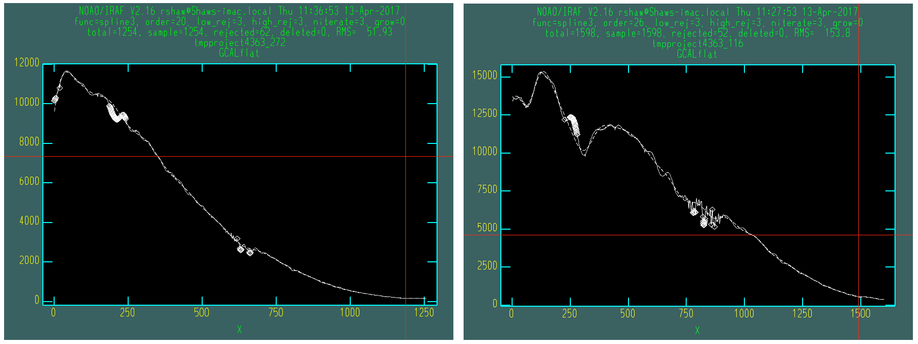
Fit to the response function of the JH (left) and HK (right) combined flat-field. A spline3 function of order 20 and 26, respectively, was used to create these normalized Flat-field MasterCals. Click image to enlarge.

5.5. Arcs

The wavelength calibration is derived from the spectrum of an arc lamp. It is common practice to take multiple arcs in the same configuration throughout an observing sequence and use the one taken closest in time to calibrate a particular frame. For this reason, the raw arc frames are not combined, even when they have the same configuration.

def selectArcs(obslog):
    arc_dict = {}
    arcFiles = obslog.file_query({'ObsType': 'ARC'})
    params = ('Texp', 'Disperser')
    for f in arcFiles:
        t, grism = obslog[f][params]
        outfile = 'arc_'+f
        arc_dict[outfile] = {'dark': 'MCdark_'+str(int(t)),
                             'flat': 'MCflat_'+grism,
                             'bpm': 'MCbpm_'+grism,
                             'input': [f]}
    return arc_dict

The selection of files for Wavelength MasterCal files is similar to that for flatfields. Each frame needs to be associated with a dark frame (of the same exposure time) and ideally a BPM file and flatfield (created using the same grism); although these are not strictly necessary, including them does improve the quality of the wavelength solution. In order to ensure the output filenames are unique, they are constructed by prepending arc_ to the raw input filename.

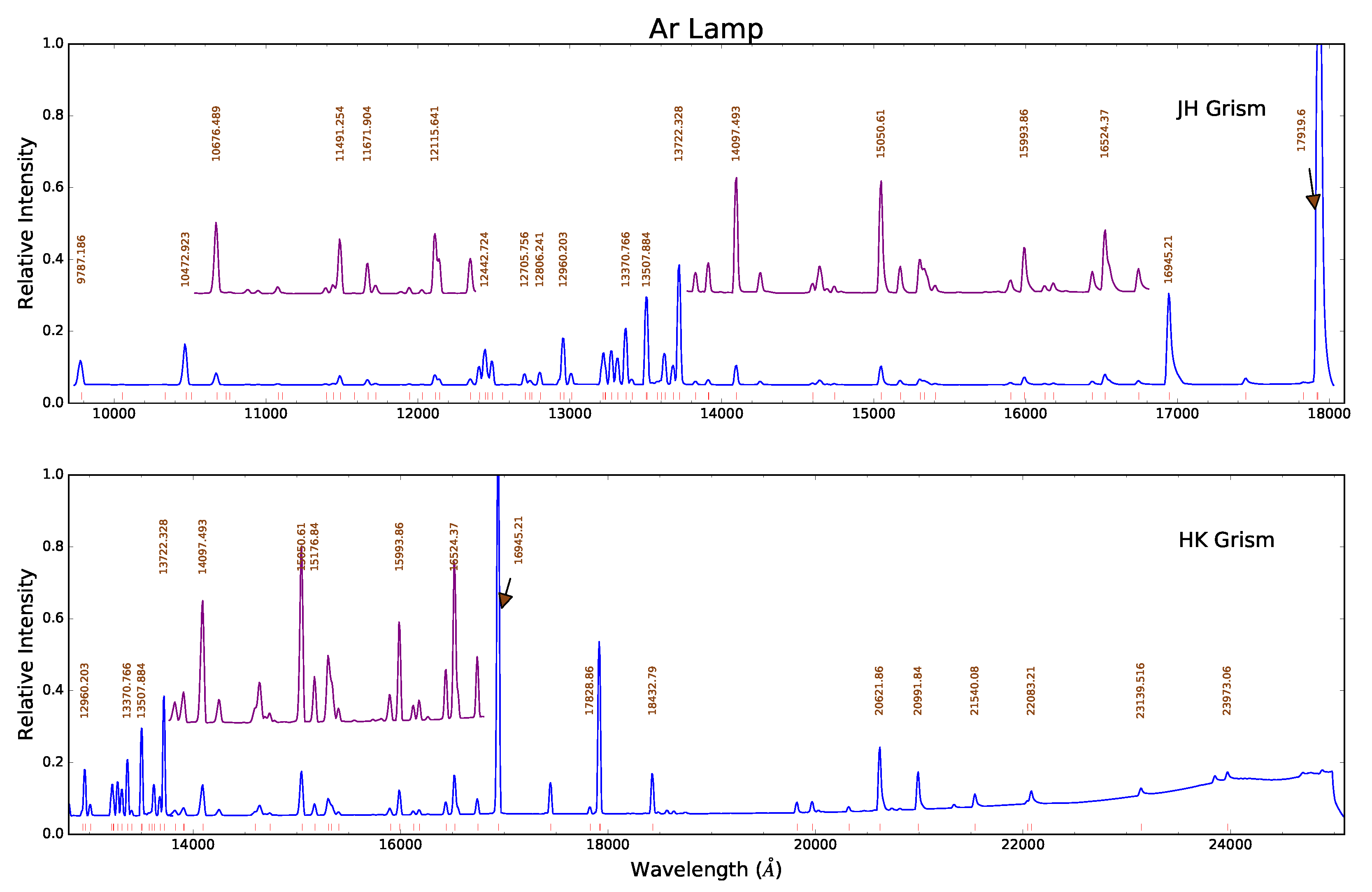
Ar spectra in the JH- band (upper) and HK- band (lower) at full scale (blue), with portions magnified (purple) and offset vertically for clarity. More than 100 identifiable lines are marked (red ticks) along the wavelength axis. Some of the brighter or more isolated lines are labeled, which should suffice to bootstrap a wavelength solution. Click image to enlarge.

def reduceArcs(arc_dict, pars):
    prepPars, arithPars, redPars, wavePars = get_pars('f2prepare', 'gemarith',
                                                    'nsreduce', 'nswavelength')
    for outfile, file_dict in arc_dict.items():
        darkFile = file_dict['dark']
        prepPars['bpm'] = file_dict['bpm']
        flatFile = file_dict['flat']
        arcFiles = file_dict['input']
        for f in arcFiles:
            f2.f2prepare(f, **prepPars)
            gemtools.gemarith('p'+f, '-', darkFile, 'dp'+f, **arithPars)
        if flatFile:
            redPars.update({'fl_flat': 'yes', 'flatimage': flatFile})
        else:
            redPars['fl_flat'] = 'no'
        gnirs.nsreduce(filelist('dp', arcFiles), **redPars)
        if len(arcFiles) > 1:
            gemcombine(filelist('rdp', arcFiles), 'tmp_'+outfile, **arithPars)
            gnirs.nswavelength('tmp_'+outfile, outspectra=outfile, **wavePars)
        else:
            gnirs.nswavelength('rdp'+arcFiles[0], outspectra=outfile,
                            **wavePars)
    iraf.imdelete('*pS*.fits')

Each entry in the previously-created dictionary is taken in turn. The input files are prepared using the associated bad pixel mask and then dark-subtracted. A call to nsreduce cuts and flatfields the frame (if a flatfield is provided). At this stage, if there are multiple input files, they are combined, before nswavelength is called to determine the wavelength solution. Intermediate files are deleted.

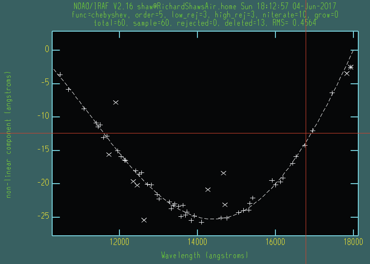
Non-linear portion of a low-order fit to the dispersion for a JH arc spectrum. A chebyshev function of order 5 should suffice to yield an RMS < 0.5. Click image to enlarge.

Due to the fixed nature of the F2 grisms, the initial wavelength solution put in the headers should be sufficiently accurate to allow IRAF to correctly identify most of the individual arc lines and it should be possible to move directly to fitting the wavelength solution, by typing f. Should the initial line identification have resulted in misidentifications, these can be deleted by moving the cursor to them and typing d. It will then be necessary to provide the correct identifications for some lines by typing m to mark an identification and entering the wavelength (in Angstroms). You should then fit a solution and can type l to have IRAF try to identify additional lines based on this new solution. More information can be obtained by typing ? and through the help pages for nswavelength and autoidentify. Like many of the IRAF tasks, the fitting is performed with the **icfit** task. Any erroneous line identifications can be deleted interactively and an appropriate order fit applied to the data. What is considered an acceptable fit depends on the grism and your scientific goals, but an rms of 0.5 Angstroms is sufficient for this tutorial.

Having determined a suitable wavelength solution, type q to quit the function fitting. The nswavelength task will now attempt to trace the arc lines along the full length of the slit, fitting a new wavelength solution at regularly-spaced intervals in order to create a distortion map across the entire image. Although you are given the option of fitting the dispersion function interactively at each stage, this is both dull and unnecessary. At the first such prompt, type NO (NB. capital letters) and you will not be asked again.

5.6. Telluric standards

The lists of telluric standards and science frames are extracted at the same time from the Target configuration file. Each reduced telluric spectrum requires a bad pixel mask, a dark frame, a flatfield, and a wavelength calibration; each reduced science spectrum requires all of those and a telluric calibration. The filenames of most of these calibrations can be determined from the properties of the input frames, but the wavelength calibration and telluric standard need to be explicitly provided.

def selectTargets(obslog):
    with open('lsTargets.yml', 'r') as yf:
        config = yaml.load(yf)
    std_dict = {}
    sci_dict = {}
    qd = {'ObsType': 'OBJECT'}
    for outfile, pars in config.items():
        infiles = obslog.file_query(merge_dicts(qd, pars))
        t, grism = obslog[infiles[0]]['Texp', 'Disperser']
        file_dict = {'dark': pars.get('dark', 'MCdark_'+str(int(t))),
                     'bpm': pars.get('bpm', 'MCbpm_'+grism),
                     'flat': pars.get('flat', 'MCflat_'+grism),
                     'arc': pars['arc'],  # Must be specified
                     'input': infiles}
        try:
            telFile = pars['telluric']
        except KeyError:  # No telluric => treat as a standard
            std_dict[outfile] = file_dict
        else:
            sci_dict[outfile] = merge_dicts(file_dict, {'telluric': telFile})
    return std_dict, sci_dict

There is one entry in the target configuration file for each output spectrum, which provides sufficient information to select the appropriate raw input files. The names of the dark, flatfield, and bad pixel mask can be provided in this file but, if absent, are constructed from the exposure time or grism. An arc must be specified. If the name of a telluric standard is not provided, then this observation is assumed to be a telluric standard itself, and it is added to the standard star reduction dictionary; otherwise it is added to the science reduction dictionary.

def reduceStandards(std_dict, pars):
    (prepPars, arithPars, fitcooPars, transPars, extrPars, redPars,
    combPars) = get_pars('f2prepare', 'gemarith', 'nsfitcoords',
                         'nstransform', 'nsextract', 'nsreduce', 'nscombine')
    redPars['fl_sky'] = 'yes'
    combPars['fl_cross'] = 'yes'
    with open('lsTargets.yml', 'r') as yf:
        config = yaml.load(yf)
    for outfile, file_dict in std_dict.items():
        darkFile = file_dict['dark']
        prepPars['bpm'] = file_dict['bpm']
        flatFile = file_dict['flat']
        arcFile = file_dict['arc']
        stdFiles = file_dict['input']
        for f in stdFiles:
            f2.f2prepare(f, **prepPars)
            gemtools.gemarith('p'+f, '-', darkFile, 'dp'+f, **arithPars)
        pars = merge_dicts(redPars, config[outfile].get('nsreduce', {}))
        gnirs.nsreduce(filelist('dp', stdFiles), flatimage=flatFile, **pars)
        gnirs.nscombine(filelist('rdp', stdFiles), output=outfile, **combPars)
        gnirs.nsfitcoords(outfile, lamptransf=arcFile, **fitcooPars)
        gnirs.nstransform('f'+outfile, **transPars)
        gnirs.nsextract('tf'+outfile, **extrPars)
        iraf.imdelete('f'+outfile+',tf'+outfile)
    iraf.imdelete('pS*.fits,dpS*.fits,rdpS*.fits')

Some of the default parameters are changed for the reduction of the standards: in particular, the individual spectra are aligned by cross-correlation before combining since the high signal-to-noise ratios makes this more accurate than using the telescope offsets.

Note

Since science targets without telluric standards have the same reduction steps as telluric standards, they are also reduced by this function. If they are too faint for cross-correlation to work, you will need to unset this flag for those objects.

The target configuration file is reopened so that any parameters required for the successful operation of nsreduce can be applied. In general, such parameters should not be required; however the interval between exposure start times for the star HD 36636 is somewhat irregular and it is necessary to set the skyrange interval for a successful reduction.

After alignment and combining, the image is transformed so that lines of constant wavelength are perfectly horizontal across the image. The task nsfitcoords fits a function to the map of the arc line spectra, and nstransform applies this to the image. There is an (optionally) interactive step to fit a 2D polynomial to the grid of datapoints, for which modest orders should suffice, especially if your science target is a point source.

The spectrum is then extracted by nsextract, which can be performed interactively. Since there will be a single bright source in the slit, the automated aperture finding and resizing routines will work well and the important step is tracing the spectrum along the wavelength direction. It may be necessary to delete points at each end (by moving to them with the cursor and pressing d) where the signal-to-noise ratio is low, to ensure that the trace is not pulled off course.

Having extracted the spectrum, you may wish to edit it to remove strong absorption features intrinsic to the standard, since these will appear as emission features in the telluric-corrected science spectra. If you do this using the splot task in IRAF then, in order to save the output, you will need to write the image to filename.fits[sci,1,overwrite].

5.7. Science targets

The dictionary to reduce the science images was constructed at the same time as the one for telluric standards and the first few reduction steps are identical, except that cross-correlation is not used to align the individual spectra. You can edit the code or the yaml parameter file if your targets are bright enough and you wish to use this method of alignment.

def reduceScience(sci_dict):
    (prepPars, arithPars, fitcooPars, transPars, extrPars, redPars, combPars,
     telPars) = get_pars('f2prepare', 'gemarith', 'nsfitcoords', 'nstransform',
                          'nsextract', 'nsreduce', 'nscombine', 'nstelluric')
    redPars['fl_sky'] = 'yes'
    with open('lsTargets.yml', 'r') as yf:
        config = yaml.load(yf)
    for outfile, file_dict in sci_dict.items():
        darkFile = file_dict['dark']
        prepPars['bpm'] = file_dict['bpm']
        flatFile = file_dict['flat']
        arcFile = file_dict['arc']
        telFile = file_dict['telluric']
        sciFiles = file_dict['input']
        for f in sciFiles:
            f2.f2prepare(f, **prepPars)
            gemtools.gemarith('p'+f, '-', darkFile, 'dp'+f, **arithPars)
        pars = merge_dicts(redPars, config[outfile].get('nsreduce', {}))
        gnirs.nsreduce(filelist('dp', sciFiles), flatimage=flatFile, **pars)
        gnirs.nscombine(filelist('rdp', sciFiles), output=outfile, **combPars)
        gnirs.nsfitcoords(outfile, lamptransf=arcFile, **nsfitcrdPars)
        gnirs.nstransform('f'+outfile, reference='xtf'+telFile, **transPars)
        pars = merge_dicts(extrPars, config[outfile].get('nsextract', {}))
        gnirs.nsextract('tf'+outfile, **pars)
        gnirs.nstelluric('xtf'+outfile, 'xtf'+telFile, **telPars)
        iraf.imdelete('f'+outfile+',tf'+outfile)
    iraf.imdelete('pS*.fits,dpS*.fits,rdpS*.fits')

To provide the best correction or atmospheric absorption features, it is important that the wavelength solutions of your science target and telluric standard are identical, so the extracted spectrum of the standard is passed to nstransform as a reference file so that the transformed science spectrum has the same dispersion. This is a new feature added to the nstransform task.

Once again, nsextract is used to produce a one-dimensional spectrum, and target-specific parameters can be provided in the target configuration file. Important parameters for this task include nsum and line, which indicate how many rows of the image to stack, and where, in order to provide a spatial profile of the slit to allow the target location(s) to be found. This tutorial involves spectroscopic observations of a brown dwarf, whose flux is heavily suppressed in substantial regions of the spectral coverage. The parameter trace is also useful if your target is faint and cannot be traced along the full wavelength range; you can set its value to the filename of a previously-extracted spectrum with a higher signal-to-noise ratio and that spectrum’s trace will be used to extract the target.

Users often report difficulty getting nstelluric to produce good results, so it may make sense to reduce your science data with the call to this task commented out so that step is not performed. You can then try running it and, if you’re not happy with the results, delete the output and try again without having to execute all the previous reduction steps.

5.8. Flux calibration

In principle, spectrophotometric calibration requires an observation of a source whose spectrum is known; however, the near-infrared spectra of stars of any given spectral type are similar enough that the telluric standard is acceptable for this task. You can find out the spectral type and apparent magnitudes of any named star using the SIMBAD search; for example, HD 36636 is an F3V star, with accurate JHK magnitudes listed. Its spectrum will therefore be very similar to that of the F3V star HD 26015 listed in the IRTF Spectral Library ([IRTF]). The spectra of stars in the near-infrared are also fairly well-modeled by blackbody spectra, and Gemini provides a list of effective temperatures, from which we deduce that HD 36636 can be represented as a blackbody with a temperature of 6680K.

There are several paths to obtaining a flux-calibrated spectrum of your target using the telluric standard, but here is one route:

1. Correct the telluric standard for atmospheric absorption in the same way as the science target.
2. Obtain/synthesize a model spectrum of the telluric standard with the same wavelength solution as your target.
3. Determine the sensitivity function (i.e., the relationship between spectral counts and flux density as a function of wavelength) using the model spectrum and the telluric-corrected standard.
4. Apply the sensitivity function to the science target, remembering to correct for the different exposure times.

These steps can all be performed with various IRAF tasks but it’s not very elegant, and there are issues interfacing the fitting task from core IRAF (continuum) that uses simple-FITS files with Gemini-IRAF tasks that use multi-extension FITS. The tutorial code includes a function, fluxCalibrate(), that performs the above steps. This requires the root filenames of the science file and telluric standard, plus a model spectrum of the standard. This can be called in one of two ways:

# Use a spectrum downloaded from the IRTF Spectral Library
fluxCalibrate('science', 'HD36636', spectrum='F3V_HD26015.txt', hmag=8.633)
# Use a blackbody spectrum
fluxCalibrate('science', 'HD36636', teff=6680, hmag=8.633)

A magnitude need not be specified if a flux-calibrated spectrum is used, but any of jmag, hmag, or kmag (Vega magnitudes) can be provided, as long as the spectrum covers that bandpass.