6. F2 MOS Tutorial
The recipe described here provides a recommended, but not unique path for processing your FLAMINGOS-2 science data. A much wider variety of calibrations are required for MOS reduction compared to the other modes offered by F2, and it may not be easy for the correct calibrations to be automatically associated with your data. You are reminded that it is possible to create or modify the reduction dictionaries as described in Python dictionaries and this may provide the simplest route to a successful data reduction experience, rather than using the automated selection functions described in this tutorial.
As a further reminder, the reduction script should be run in segments, only uncommenting the two or three lines needed to perform each of the following steps during each execution of the script, and the results should be inspected after each step.
The data in this tutorial comprise J and K-band spectra of the Galactic star-forming region S5, taken as part of the MOS science verification (SV) program.
6.1. Retrieving the Data
The first step is to retrieve the data from the Gemini Observatory Archive (see Archive Searches). To download the data for this tutorial, the following URL should be pasted into your browser:
Click the button at the bottom of the page labeled “Download all 309 files
totalling 1.03 GB”. To ease the reduction, it makes sense to separate the
July (J-band) and August (K-band) datasets, so you should make two separate
directories (called J and K, or July and August, for example)
and create subdirectories named raw in each of these. The raw FITS files
should be extracted by unzipping the downloaded zip file and then separated.
The program includes some daytime flatfields taken through the slit mask but
the F2 instrument team has decided that nighttime flats should be used in the
reduction, so these files are surplus to requirements and can therefore
be deleted, together with a few other extraneous files.
rm July/raw/S20190701S005*
rm July/raw/S20190703S*
rm July/raw/S20190707S*
rm August/S20190810S*
As this is an SV program, it includes most of the required calibrations; however, it lacks proximate 80-second darks for the J-band telluric standard, and 7-second darks for the K-band MOS flats (the 9-second darks are too bright and in the highly non-linear regime). These can be obtained by clicking on “Load Associated Calibrations” and selecting the sets of darks indicated by an asterisk in the table below.
6.1.1. Exposure Summary
| Sequence numbers | Target | Waveband | T_exp | N_exp |
|---|---|---|---|---|
| S20190701S0060-0069 | HD 152602 | J | 80 | 10 |
| S20190701S0070 | Flat | J | 20 | 1 |
| S20190701S0071 | Arc | J | 30 | 1 |
| S20190701S0080 | Flat | J | 20 | 1 |
| S20190701S0081 | Arc | J | 30 | 1 |
| S20190701S0082-0089 | S5 | J | 300 | 8 |
| S20190701S0090 | Flat | J | 20 | 1 |
| S20190701S0091 | Arc | J | 30 | 1 |
| S20190701S0092-0099 | S5 | J | 300 | 8 |
| S20190701S0100 | Flat | J | 20 | 1 |
| S20190701S0101 | Arc | J | 30 | 1 |
| S20190702S0624-0634 | Dark | 2 | 11 | |
| S20190702S0635-0645 | Dark | 10 | 11 | |
| S20190702S0646-0656 | Dark | 20 | 11 | |
| S20190702S0657-0667 | Dark | 30 | 11 | |
| S20190702S0668-0677 | Dark | 300 | 10 | |
| S20190702S0678-0684 | Dark | 30 | 7 | |
| S20190702S0685-0691 | Dark | 20 | 7 | |
| S20190706S0368-0374 | Dark* | 80 | 7 | |
| S20190809S0082-0092 | HD 152602 | K | 80 | 11 |
| S20190809S0093-0097 | Flat | K | 9 | 5 |
| S20190809S0098 | Arc | K | 80 | 1 |
| S20190809S0099 | Flat | K | 80 | 1 |
| S20190809S0107-0111 | Flat | K | 9 | 5 |
| S20190809S0112 | Arc | K | 80 | 1 |
| S20190809S0113 | Flat | K | 80 | 1 |
| S20190809S0114-0121 | S5 | K | 300 | 8 |
| S20190809S0122-0125 | Flat | K | 7 | 4 |
| S20190809S0126 | Flat | K | 9 | 1 |
| S20190809S0127 | Arc | K | 80 | 1 |
| S20190809S0128 | Flat | K | 80 | 1 |
| S20190809S0232-0240 | Dark | 2 | 9 | |
| S20190809S0241-0249 | Dark | 10 | 9 | |
| S20190809S0250-0258 | Dark | 9 | 9 | |
| S20190809S0259-0267 | Dark | 80 | 9 | |
| S20190809S0268-0276 | Dark | 300 | 9 | |
| S20190811S0339-0345 | Dark* | 7 | 7 |
6.2. Preparation
First download obslog.py to the
July/raw subdirectory and create an observing log, as described in
Observing Log.
python obslog.py obslog.fits
Copy the obslog.py file to the August/raw directory and run the
same command there to produce an observing log for August.
The other files needed for this tutorial are a python script and two configuration files.
- Download:
reduce_mos.py
Configuration files are required for the IRAF task parameters that differ from the defaults, and to provide the script with information about the targets.
- Download IRAF task parameters:
mosTaskPars.yml - Download target information:
mosTargets_July.ymlmosTargets_August.yml
Identical copies of the reduce_mos.py and mosTaskPars.yml` files should
be placed in each of the July and August directories, while the two
files with target information should be placed in the relevant directories and
both renamed simply to mosTargets.yml.
mv mosTargets_July.yml July/mosTargets.yml
mv mosTargets_August.yml August/mosTargets.yml
6.2.1. Target configuration files
We need two two target configuration files, one for July/J and one for August/K, which look like this:
# Attributes of observed targets for the 2019-Jul observing run.
#
HD152602J:
    first:     S20190701S0060
    last:      S20190701S0063
    arc:       arc_S20190701S0071

S5_J1:
    first:     S20190701S0082
    last:      S20190701S0089
    arc:       arc_S20190701S0081
    flat:      flat_S20190701S0080
    telluric:  HD152602J

S5_J2:
    first:     S20190701S0092
    last:      S20190701S0099
    arc:       arc_S20190701S0091
    flat:      flat_S20190701S0090
    telluric:  HD152602J
# Attributes of observed targets for the 2019-Aug observing run.
#
HD152602K:
    Object:    HD 152602
    first:     S20190809S0083
    arc:       arc_S20190809S0098
    Filter:    K-long

S5_K:
    Object:    S5
    Date:      20190809
    arc:       arc_S20190809S0127
    flat:      flat_S20190809S0122_0125
    telluric:  HD152602K
6.2.2. Configuration of nsreduce
he nsreduce task has several parameters; the table below lists
the defaults for the processing flags — i.e., the parameters with
logical values to indicate whether to perform an operation. Since
each task is unlearned before being run, only parameters that differ
from the defaults need to be specified in the mosTaskPars.yml
file.
| Flag | Default | Description |
|---|---|---|
fl_cut |
Yes | Cut images using F2CUT? |
fl_process_cut |
Yes | Cut the data before processing? |
fl_nsappwave |
Yes | Insert approximate wavelength WCS keywords into header? |
fl_dark |
No | Subtract dark image? |
fl_save_dark |
No | Save processed dark files? |
fl_sky |
No | Perform sky subtraction using skyimages? |
fl_flat |
Yes | Apply flat-field correction? |
fl_vardq |
Yes | Propagate VAR and DQ? |
The parameter values need to be chosen carefully, as the order of operations performed by the task is not consistent with the order adopted in this tutorial. This means nsreduce will be invoked multiple times, with different flag settings, to accomplish the processing steps in the needed order.
6.3. Darks
Since dark frames are the same irrespective of whether they are used for imaging or spectroscopic observations, the procedure for reducing them is identical to that described in the Imaging Tutorials’ section on Darks.
A helper function, check_cals(), is provided to confirm that all
the necessary calibration files in a reduction dictionary exist in
the current directory. If any are missing, their names
will be reported and the script will exit immediately, rather than
proceeding up to the point where the missing calibration is needed.
It is suggested that this
function always be called immediately before any reduction step.
6.4. Flatfields
The dataset includes both longslit flats, which are used to reduce the telluric standard, and MOS flats taken through the slit mask, which are used to reduce the science data.
Since the reduction steps for each type of flat are different,
the selectFlats() function returns two dict objects, one for the
longslit flats, and one for the MOS flats, which are identified from the
name of the slit mask in the header. It attempts to provide sensible
default behavior, but you are advised to check its output to understand how
it is producing the flatfields. Note, for example, that it is not possible
to combine frames with different exposure times with this code, because such
frames require different darks.
def selectFlats(obslog):
    # key=(output flat, output bpm); value=[dark, [input files]]
    ls_flat_dict = {}
    mos_flat_dict = {}
    qd = {'ObsType': 'FLAT', 'GCAL Shutter': 'OPEN'}
    params = ('Texp', 'Disperser', 'Mask', 'Filter', 'Date')
    flatConfigs = unique(obslog.query(qd)[params])
    for config in flatConfigs:
        t, grism, mask, filt, date = config
        config_dict = dict(zip(params, config))
        flatFiles = sorted(obslog.file_query(merge_dicts(qd, config_dict)))
        # This format for MCdark files is suitable for nightly darks
        file_dict = {'dark': 'MCdark_'+str(int(t)),
                     'bpm': 'MCbpm_{}_{}.pl'.format(grism, filt)}

        if 'pix-slit' in mask:
            # Long-slit flat (for standard) -- create BPM
            outfile = '_'.join(['MCflat', grism, filt])
            file_dict['input'] = flatFiles
            ls_flat_dict[outfile] = file_dict.copy()
        else:
            # Find groups of flats and combine each group
            for infiles in make_contiguous_lists(flatFiles):
                file_dict['input'] = infiles
                seq = infiles[0]
                if len(infiles) > 1:
                    seq += "_"+infiles[-1][-4:]
                outfile = 'flat_'+seq
                slitFile = 'slits_'+seq
                mos_flat_dict[outfile] = merge_dicts(file_dict,
                                                     {'slitim': slitFile})
    return ls_flat_dict, mos_flat_dict
6.4.1. Longslit flatfields
The bad pixel mask (BPM) will be created during the reduction of the longslit
flats. For this reason, longslit flats should always be reduced before the
MOS flats. Since both the J and K-band spectra are taken with the R3K grism,
the flatfields are assigned the name MCflat_<grism>_<filter>.fits.
If there are multiple exposure times and/or
slit widths among the raw flats for a particular grism, then the master flat
will be created from only one of these combinations; this will be the last
one encountered which will not be reproducible from run to run given the
unordered nature of python dict structures. Therefore you should deselect
the use_me flag for all but one such combination, or edit the code to
produce a unique filename for each combination. See Flatfields for more
details.
Here we have two longslit K-band flats, one each on the nights of August 9
and 10. By default these would both be assigned the output filename
MCflat_R3K_K-long and so only one will be created. For the purposes of
this tutorial, that’s OK but you may wish to create two separate flatfields
with different filenames.
6.4.2. MOS flatfields
MOS flatfields are taken in batches before and after the science observations, and each batch is reduced separately and given a unique name based on the start and end observation filenames.
def reduceMOSFlats(flat_dict):
    prepPars, cutPars, arithPars, flatPars, combPars, sdistPars = get_pars('f2prepare',
                                'f2cut', 'gemarith', 'nsflat', 'gemcombine', 'nssdist')
    for outfile, file_dict in flat_dict.items():
        darkFile = file_dict['dark']
        bpmFile = file_dict['bpm']
        slitFile = file_dict['slitim']
        refImage = file_dict.get('reference', '')
        flatFiles = file_dict['input']
        nsflat_inputs = filelist('cdp', flatFiles)
        for f in flatFiles:
            f2.f2prepare(f, **merge_dicts(prepPars, {'bpm': bpmFile}))
            gemtools.gemarith('p'+f, '-', darkFile, 'dp'+f, **arithPars)
        if not refImage:
            if len(flatFiles) > 1:
                # Stack images and use this to make reference
                gemtools.gemcombine(filelist('dp', flatFiles), 'stack', **combPars)
                cutPars.update({'gradimage': 'stack',
                                'refimage': '', 'outslitim': slitFile})
                f2.f2cut('stack', outimages='cut_'+outfile, **cutPars)
                # Use the cut stack as a reference for individual images
                cutPars.update({'gradimage': '', 'refimage': 'cut_'+outfile})
                f2.f2cut(filelist('dp', flatFiles), **cutPars)
            else:
                # If only one image, use it to cut itself and ensure it
                # has an appropriate name
                cutPars.update({'gradimage': 'dp'+flatFiles[0],
                                'refimage': '', 'outslitim': slitFile})
                f2.f2cut(filelist('dp', flatFiles), outimages='cut_'+outfile,
                         **cutPars)
                nsflat_inputs = 'cut_'+outfile
            gnirs.nssdist(slitFile, **sdistPars)
        else:
            cutPars.update({'gradimage': '', 'refimage': refImage})
            f2.f2cut(filelist('dp', flatFiles), **cutPars)

        flatPars.update({'flatfile': outfile, 'bpmfile': ''})
        gnirs.nsflat(nsflat_inputs, **flatPars)

        iraf.imdelete('stack.fits')
    iraf.imdelete('pS*.fits,dpS*.fits,cdpS*.fits')
In addition to the flatfield, it’s also necessary to have a reference file
which contains the modified MDF from f2cut (containing information about
the regions of the image corresponding to each slit) as this is not propagated
by nsflat. This file (which is simply the un-normalized flatfield) is given
the same name as the flatfield, with the prefix cut_.
At this time, it is worth considering whether you
wish to reduce all the flatfields; for example, three flats are taken on
July 1 to support the J-band observations of the target. There’s no harm in
reducing all of these but, if you choose to fit them interactively,
it will take some time. Uncomment the lines indicated in the reduce_mos.py
script.
The individual slit spectra are extracted over the full range of the wavelength coverage and therefore warnings will appear that the “DQ for flat is poor”, indicating that the signal is low. These are nothing to worry about. While reducing the flats, you will note that slits 38 and 49 both have regions where the signal dips. What are these? A detector defect?
6.5. Arcs
As with the flatfields, two arc reduction dictionaries are constructed by the
selectArcs() function: one from the longslit data to reduce the telluric
standards, and one from the MOS data to reduce the science observations.
However, both dictionaries are reduced by the same function, reduceArcs().
def selectArcs(obslog):
    with open('mosTargets.yml', 'r') as yf:
        config = yaml.load(yf)

    ls_arc_dict = {}
    mos_arc_dict = {}
    arcFiles = obslog.file_query({'ObsType': 'ARC'})
    params = ('Texp', 'Disperser', 'Mask', 'Filter')
    # Do not stack arcs; reduce each separately
    for f in arcFiles:
        t, grism, mask, filt = obslog[f][params]
        file_dict = {'dark': 'MCdark_'+str(int(t)),
                     'bpm': 'MCbpm_{}_{}'.format(grism, filt),
                     'input': [f]}
        outfile = 'arc_'+f

        possible_flats = obslog.file_query({'ObsType': 'FLAT',
                                            'GCAL Shutter': 'CLOSED',
                                            'Texp': t})
        for flat in possible_flats:
            if flat[:10] == f[:10] and abs(int(flat[10:])-int(f[10:])) == 1:
                file_dict['dark'] = flat
                break

        if 'pix-slit' in mask:
            file_dict['flat'] = 'MCflat_{}_{}'.format(grism, filt)
            ls_arc_dict[outfile] = file_dict.copy()
        else:
            for sci_dict in config.values():
                if sci_dict.get('arc') == outfile:
                    # Use the same flat for this arc as the science frame
                    # it's going to calibrate
                    flatFile = sci_dict['flat']
                    file_dict['flat'] = flatFile
                    file_dict['slits'] = flatFile.replace('flat_', 'slits_')
                    file_dict['reference'] = 'cut_'+flatFile
                    mos_arc_dict[outfile] = file_dict.copy()
                    break
    return ls_arc_dict, mos_arc_dict
The wavelength calibration in the K-band is often more successful
if the thermal continuum emission is subtracted from the arc lamp spectrum.
Such exposures are taken as lamp-off flats, but should be treated as if
they are darks. The selectArcs() function tries to deal with this by
looking for a flat with the same exposure time and setting as each arc and
a sequence number that differs only by one, indicating it was taken either
immediately before or immediately after the arc.
If your data do not follow this pattern, you may need to manually assign
an appropriate exposure if there is no suitable MCdark file.
def reduceArcs(arc_dict):
    prepPars, arithPars, redPars, fitcrdPars, transPars = get_pars('f2prepare',
                         'gemarith', 'nsreduce', 'nsfitcoords', 'nstransform')
    for outfile, file_dict in arc_dict.items():
        (wavePars,) = get_pars('nswavelength')
        darkFile = file_dict['dark']
        flatFile = file_dict.get('flat')
        slitsFile = file_dict.get('slits')
        refFile = file_dict.get('reference', '')
        bpmFile = file_dict['bpm']
        arcFiles = file_dict['input']
        for f in arcFiles:
            f2.f2prepare(f, **merge_dicts(prepPars, {'bpm': bpmFile}))
            # K-band arcs may have a single exposure to remove thermal emission
            # so that exposure will need to be prepared
            if darkFile.startswith('S20'):
                f2.f2prepare(darkFile, **merge_dicts(prepPars, {'bpm': bpmFile}))
                darkFile = 'p'+darkFile
            gemtools.gemarith('p'+f, '-', darkFile, 'dp'+f, **arithPars)
        # Flatfields not required for arcs
        if flatFile:
            redPars.update({'fl_flat': 'yes', 'flatimage': flatFile})
        else:
            redPars['fl_flat'] = 'no'
        redPars['refimage'] = refFile
        gnirs.nsreduce(filelist('dp', arcFiles), **redPars)
        if len(arcFiles) > 1:
            arc = 'tmp_'+outfile
            gemcombine(filelist('rdp', arcFiles), arc, **arithPars)
        else:
            arc = 'rdp'+arcFiles[0]
        if slitsFile:
            gnirs.nsfitcoords(arc, sdisttransf=slitsFile, **fitcrdPars)
            gnirs.nstransform('f'+arc, **transPars)
            iraf.imdelete(arc+',f'+arc)
            arc = 'tf'+arc
            wavePars.update({'step': 5})
        gnirs.nswavelength(arc, outspectra=outfile, **wavePars)
        iraf.imdelete(arc)
    iraf.imdelete('*pS*.fits,dpS*.fits')
6.5.1. Longslit arcs
Longslit arcs are reduced in the manner described in Arcs. See that section for more details.
6.5.2. MOS arcs
In a normal observing sequence, arcs will be taken through the MOS mask immediately before and after each sequence of science observations, but only one of these will be used to wavelength-calibrate the data. Which one you use shouldn’t matter, as they should be very similar, but it is probably worth using each one in a separate reduction and comparing the results.
Only the MOS arcs that are listed in the mosTargets.yml file will be
reduced. The reduction stars with cutting the separate slits and straightening
them using the traces from the flatfield, which can take a little while. Once
that has been completed, each slit has to be calibrated independently and,
as with the longslit reduction, you will first be asked whether you wish to
fit the wavelength solution for the middle column interactively and, once you
are satisfied with that, you will be asked if you wish to interactively fit
the solution for columns on either side as the arc lines are traced
outward towards the edges of each slit. You can happily answer ‘NO’ to this
second question but the initial wavelength solutions should always be
determined interactively in case one or more of the slits fails to produce
the correct solution. In this tutorial, 103 slits from three MOS arcs
are reduced and only slit 22 of S20190701S0081 fails to produce the
correct solution automatically.
6.6. Telluric standards
Telluric standards are taken though the longslit and their reduction is therefore
identical to that described in Telluric standards. Each standard must have an
entry in the mosTargets.yml file that defines the input frames and also the
arc to use for wavelength calibration.
6.7. Science targets
Each entry in the mosTargets.yml file that corresponds to a science target
must be provided with a flatfield and a reduced telluric standard in addition to
an arc. Even if you do not intend to perform a telluric correction, the telluric
standard is required to define the output wavelength solution to which
nstransform will resample each slit’s spectrum. As with longslit reduction,
it may be advantageous to reduce the science targets without running
nstelluric (by commenting out this line in the reduceScience() function)
so you will not have to repeat the reduction (which is quite slow)
if the telluric correction is not as successful as you require.
The same telluric correction will be applied to all spectra, so this should be
determined from one of the MOS spectra with a high signal-to-noise ratio. For
historical reasons, the parameter named ifuextn in nstelluric controls
which slit is used to determine the telluric correction, and this should therefore
be defined in the mosTaskPars.yml file to correspond to a high-SNR spectrum
in the science data. Alternatively, this parameter can be set to zero and each
spectrum in the science data will be processed separately, but this is not
advised unless you have a high signal-to-noise ratio in all your spectra.
In addition to the standard reduceScience() function used in this tutorial,
there is a function called
reduceABBAScience(). This is suitable for observations were the telescope is
nodded between only two positions (either both within the slit or one being an
offset to sky), and follows a slightly different reduction
procedure that may produce better results. It stacks each set of images before
subtracting one set from the other and then transforming the slits. If the two
telescope positions are close together on the sky, then the two stacks are
subsequently aligned and added together. This has not been extensively tested.
6.8. Flux calibration
This follows the same procedure as described in Flux calibration so the J and K-band spectra should be flux calibrated with the commands
fluxCalibrate('S5_J1', 'HD152602J', jmag=9.536, teff=10700)
fluxCalibrate('S5_J2', 'HD152602J', jmag=9.536, teff=10700)
fluxCalibrate('S5_K', 'HD152602K', kmag=9.396, teff=10700)
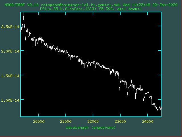
K-band spectrum of slit 16, after flux calibration. The units of the plot are Angstroms and erg cm-2 s-1 A-1.
6.9. Outstanding issues
The spectral resolution of F2 varies across the image, which can result in a poor telluric correction for those MOS spectra whose resolution differs most greatly from the longslit telluric standard. If this is likely to cause problems, the telluric can be nodded along the full length of the longslit (as has been done here) and separate groups combined to produce multiple spectra (which is not done here). The science data can then be telluric-corrected with each of these and the best output spectrum chosen on a slit-by-slit basis.